
A Decision Tree is a powerful and popular machine learning algorithm used for both classification and regression tasks. It is a graphical representation of a series of decisions and their possible outcomes, making it easy to understand and interpret. The ID3 (Iterative Dichotomiser 3) algorithm is one of the earliest and most widely used algorithms to create decision trees from a given dataset. In this blog, we will walk through the steps of creating a decision tree using the ID3 algorithm with a solved example.
What is Decission Tree?
A Decision Tree is a popular machine learning algorithm used for both classification and regression tasks. It is a tree-like structure that represents a series of decisions and their possible outcomes. Each internal node of the tree corresponds to a feature or attribute, each branch represents a decision based on that attribute, and each leaf node represents the final outcome or class label. Decision Trees are interpretable and easy to understand, making them useful for both analysis and prediction.
What is ID3 Algorithm?
The ID3 (Iterative Dichotomiser 3) algorithm is one of the earliest and most widely used algorithms to create Decision Trees from a given dataset. It uses the concept of entropy and information gain to select the best attribute for splitting the data at each node. Entropy measures the uncertainty or randomness in the data, and information gain quantifies the reduction in uncertainty achieved by splitting the data on a particular attribute. The ID3 algorithm recursively splits the dataset based on the attributes with the highest information gain until a stopping criterion is met, resulting in a Decision Tree that can be used for classification tasks.
Understanding the ID3 Algorithm:
The ID3 algorithm uses the concept of entropy and information gain to construct a decision tree. Entropy measures the amount of uncertainty or randomness in a dataset, while information gain quantifies the reduction in entropy achieved by splitting the data on a specific attribute. The attribute with the highest information gain is selected as the decision node for the tree.
Steps to Create a Decision Tree using the ID3 Algorithm:
Step 1: Data Preprocessing:
Clean and preprocess the data. Handle missing values and convert categorical variables into numerical representations if needed.
Step 2: Selecting the Root Node:
Calculate the entropy of the target variable (class labels) based on the dataset. The formula for entropy is:Entropy(S) = -Σ (p_i * log2(p_i))
where p_i is the proportion of instances belonging to class i.
Step 3: Calculating Information Gain:
For each attribute in the dataset, calculate the information gain when the dataset is split on that attribute. The formula for information gain is:Information Gain(S, A) = Entropy(S) - Σ ((|S_v| / |S|) * Entropy(S_v))
where S_v is the subset of instances for each possible value of attribute A, and |S_v| is the number of instances in that subset.
Step 4: Selecting the Best Attribute:
Choose the attribute with the highest information gain as the decision node for the tree.
Step 5: Splitting the Dataset:
Split the dataset based on the values of the selected attribute.
Step 6: Repeat the Process:
Recursively repeat steps 2 to 5 for each subset until a stopping criterion is met (e.g., the tree depth reaches a maximum limit or all instances in a subset belong to the same class).
Solved Example:
Let’s illustrate the ID3 algorithm with a simple example of classifying whether to play tennis based on weather conditions. Consider the following dataset:
| Weather | Temperature | Humidity | Windy | Play Tennis? |
|---|---|---|---|---|
| Sunny | Hot | High | False | No |
| Sunny | Hot | High | True | No |
| Overcast | Hot | High | False | Yes |
| Rainy | Mild | High | False | Yes |
| Rainy | Cool | Normal | False | Yes |
| Rainy | Cool | Normal | True | No |
| Overcast | Cool | Normal | True | Yes |
| Sunny | Mild | High | False | No |
| Sunny | Cool | Normal | False | Yes |
| Rainy | Mild | Normal | False | Yes |
| Sunny | Mild | Normal | True | Yes |
| Overcast | Mild | High | True | Yes |
| Overcast | Hot | Normal | False | Yes |
| Rainy | Mild | High | True | No |
Step 1: Data Preprocessing:
The dataset does not require any preprocessing, as it is already in a suitable format.
Step 2: Calculating Entropy:
To calculate entropy, we first determine the proportion of positive and negative instances in the dataset:
- Positive instances (Play Tennis = Yes): 9
- Negative instances (Play Tennis = No): 5
Entropy(S) = -(9/14) * log2(9/14) – (5/14) * log2(5/14) ≈ 0.940
Step 3: Calculating Information Gain:
We calculate the information gain for each attribute (Weather, Temperature, Humidity, Windy) and choose the attribute with the highest information gain as the root node.
Information Gain(S, Weather) = Entropy(S) – [(5/14) * Entropy(Sunny) + (4/14) * Entropy(Overcast) + (5/14) * Entropy(Rainy)] ≈ 0.246
Information Gain(S, Temperature) = Entropy(S) – [(4/14) * Entropy(Hot) + (4/14) * Entropy(Mild) + (6/14) * Entropy(Cool)] ≈ 0.029
Information Gain(S, Humidity) = Entropy(S) – [(7/14) * Entropy(High) + (7/14) * Entropy(Normal)] ≈ 0.152
Information Gain(S, Windy) = Entropy(S) – [(8/14) * Entropy(False) + (6/14) * Entropy(True)] ≈ 0.048
Step 4: Selecting the Best Attribute:
The “Weather” attribute has the highest information gain, so we select it as the root node for our decision tree.
Step 5: Splitting the Dataset:
We split the dataset based on the values of the “Weather” attribute into three subsets (Sunny, Overcast, Rainy).
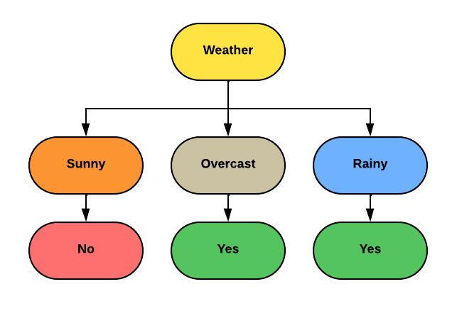
Step 6: Repeat the Process:
Since the “Weather” attribute has n0o repeating values in any subset, we stop splitting and label each leaf node with the majority class in that subset. The decision tree will look like below:
Python code for creating a decision tree using the ID3 algorithm:
import pandas as pd
import numpy as np
import random

# Define the dataset
data = {
    'Weather': ['Sunny', 'Sunny', 'Overcast', 'Rainy', 'Rainy', 'Rainy', 'Overcast', 'Sunny', 'Sunny', 'Rainy', 'Sunny', 'Overcast', 'Overcast', 'Rainy'],
    'Temperature': ['Hot', 'Hot', 'Hot', 'Mild', 'Cool', 'Cool', 'Cool', 'Mild', 'Cool', 'Mild', 'Mild', 'Mild', 'Hot', 'Mild'],
    'Humidity': ['High', 'High', 'High', 'High', 'Normal', 'Normal', 'Normal', 'High', 'Normal', 'Normal', 'Normal', 'High', 'Normal', 'High'],
    'Windy': [False, True, False, False, False, True, True, False, False, False, True, True, False, True],
    'Play Tennis': ['No', 'No', 'Yes', 'Yes', 'Yes', 'No', 'Yes', 'No', 'Yes', 'Yes', 'Yes', 'Yes', 'Yes', 'No']
}

df = pd.DataFrame(data)

def entropy(target_col):
    elements, counts = np.unique(target_col, return_counts=True)
    entropy_val = -np.sum([(counts[i] / np.sum(counts)) * np.log2(counts[i] / np.sum(counts)) for i in range(len(elements))])
    return entropy_val

def information_gain(data, split_attribute_name, target_name):
    total_entropy = entropy(data[target_name])
    vals, counts= np.unique(data[split_attribute_name], return_counts=True)
    weighted_entropy = np.sum([(counts[i] / np.sum(counts)) * entropy(data.where(data[split_attribute_name]==vals[i]).dropna()[target_name]) for i in range(len(vals))])
    information_gain_val = total_entropy - weighted_entropy
    return information_gain_val

def id3_algorithm(data, original_data, features, target_attribute_name, parent_node_class):
    # Base cases
    if len(np.unique(data[target_attribute_name])) <= 1:
        return np.unique(data[target_attribute_name])[0]
    elif len(data) == 0:
        return np.unique(original_data[target_attribute_name])[np.argmax(np.unique(original_data[target_attribute_name], return_counts=True)[1])]
    elif len(features) == 0:
        return parent_node_class
    else:
        parent_node_class = np.unique(data[target_attribute_name])[np.argmax(np.unique(data[target_attribute_name], return_counts=True)[1])]
        item_values = [information_gain(data, feature, target_attribute_name) for feature in features]
        best_feature_index = np.argmax(item_values)
        best_feature = features[best_feature_index]
        tree = {best_feature: {}}
        features = [i for i in features if i != best_feature]
        for value in np.unique(data[best_feature]):
            value = value
            sub_data = data.where(data[best_feature] == value).dropna()
            subtree = id3_algorithm(sub_data, data, features, target_attribute_name, parent_node_class)
            tree[best_feature][value] = subtree
        return tree

def predict(query, tree, default = 1):
    for key in list(query.keys()):
        if key in list(tree.keys()):
            try:
                result = tree[key][query[key]]
            except:
                return default
            result = tree[key][query[key]]
            if isinstance(result, dict):
                return predict(query, result)
            else:
                return result

def train_test_split(df, test_size):
    if isinstance(test_size, float):
        test_size = round(test_size * len(df))
    indices = df.index.tolist()
    test_indices = random.sample(population=indices, k=test_size)
    test_df = df.loc[test_indices]
    train_df = df.drop(test_indices)
    return train_df, test_df

train_data, test_data = train_test_split(df, test_size=0.2)

def fit(df, target_attribute_name, features):
    return id3_algorithm(df, df, features, target_attribute_name, None)

def get_accuracy(df, tree):
    df["classification"] = df.apply(predict, axis=1, args=(tree, 'Yes'))
    df["classification_correct"] = df["classification"] == df["Play Tennis"]
    accuracy = df["classification_correct"].mean()
    return accuracy

tree = fit(train_data, 'Play Tennis', ['Weather', 'Temperature', 'Humidity', 'Windy'])
accuracy = get_accuracy(test_data, tree)
print("Decision Tree:")
print(tree)
print("Accuracy:", accuracy)
Output:
Decision Tree: {'Weather': {'Overcast': 'Yes', 'Rainy': {'Windy': {False: 'Yes', True: 'No'}}, 'Sunny': {'Temperature': {'Cool': 'Yes', 'Hot': 'No', 'Mild': 'No'}}}}
Accuracy: 0.6666666666666666
Limitations of the ID3 Algorithm and Decision Trees:
While decision trees and the ID3 algorithm offer several advantages, they also have some limitations that need to be considered before using them in certain scenarios:
- Overfitting: Decision trees are prone to overfitting, especially when the tree becomes too deep or complex. Overfitting occurs when the tree captures noise or random fluctuations in the training data, leading to poor performance on unseen data.
- Instability: Small changes in the data can lead to different tree structures, making decision trees less stable. A small variation in the data might cause a split at a different attribute or threshold, potentially affecting the entire tree.
- Inability to Capture Linear Relationships: Decision trees are not well-suited to capture linear relationships between variables. They partition the data into distinct regions, making it challenging to represent linear patterns.
- Bias towards Features with More Levels: Attributes with more levels or categories tend to have higher information gain simply due to having more possible splits. This can bias the decision tree towards such attributes, even if they might not be the most informative.
- Lack of Robustness to Noise: Decision trees can be sensitive to noisy data, as they might create splits based on noise or outliers that do not generalize well to new data.
- Difficulty in Handling Continuous Variables: The ID3 algorithm and basic decision trees are designed to handle categorical variables. For continuous variables, pre-processing is required to convert them into discrete intervals or use other algorithms like CART (Classification and Regression Trees).
- Exponential Growth of Tree Size: Decision trees can grow rapidly, especially when dealing with large datasets or a high number of features. This can lead to complex trees that are difficult to interpret.
- Limited Expressiveness: While decision trees can represent simple decision boundaries, they might struggle to capture complex relationships in the data.
- Difficulty in Handling Missing Values: The ID3 algorithm does not handle missing values well. Imputation methods or other algorithms need to be used to handle missing data.
- Class Imbalance: Decision trees can have difficulty dealing with imbalanced class distributions in the data, potentially favoring the majority class and performing poorly on the minority class.
Despite these limitations, decision trees and the ID3 algorithm remain widely used and can still be effective in various scenarios, especially when combined with techniques like pruning, ensemble methods (e.g., Random Forests, Gradient Boosting), or when used as part of more sophisticated machine learning pipelines. Understanding the strengths and weaknesses of decision trees helps data scientists and machine learning practitioners make informed decisions about their use in different applications.
Conclusion:
In this blog, we walked through the steps of creating a decision tree using the ID3 algorithm with a solved example. The ID3 algorithm is an effective way to build decision trees by selecting the best attribute at each node based on information gain. Decision trees are intrpretable, easy to understand, and can be used for various classification tasks.
Find this tutorial on Github.