
In the ever-evolving world of technology, machine learning has become a powerful tool to tackle various real-world challenges. One such application is predicting house prices using linear regression for real estate. The ability to forecast property values can immensely benefit real estate agents, homeowners, and buyers alike. In this blog, we will explore a fascinating machine learning project that leverages the linear regression algorithm to predict house sale prices accurately using python.
Understanding Linear Regression:
Linear regression is a fundamental supervised learning algorithm in machine learning. It aims to establish a linear relationship between a dependent variable (target) and one or more independent variables (features). In the context of house price prediction, the dependent variable will be the house price, and the independent variables can be factors like the size of the house, number of bedrooms, location, etc.
House Price Prediction with Linear Regression Involves Following Steps:
- Dataset Collection: Gather historical house price data and corresponding features from platforms like Zillow or Kaggle.
- Data Preprocessing: Clean the data, handle missing values, and perform feature engineering, such as converting categorical variables to numerical representations.
- Splitting the Dataset: Divide the dataset into training and testing sets for model building and evaluation.
- Building the Model: Create a linear regression model to learn the relationships between features and house prices.
- Model Evaluation: Assess the model’s performance on the testing set using metrics like MSE or RMSE.
- Fine-tuning the Model: Adjust hyperparameters or try different algorithms to improve the model’s accuracy.
- Deployment and Prediction: Deploy the robust model into a real-world application for predicting house prices based on user inputs.
House Price Prediction Project in Python Source Code
For this project we will be a house dataset which will be having columns – date, price, bedrooms, bathrooms, sqft_living, sqft_lot, floors, waterfront, view, condition. You can download the dataset from here.
Step1: Dataset Exploration and Preprocessing:
import pandas as pd
import matplotlib.pyplot as plt
import seaborn as sns
from sklearn.model_selection import train_test_split
from sklearn.linear_model import LinearRegression
from sklearn.metrics import mean_squared_error, r2_score

# Load the dataset from CSV
df = pd.read_csv('house_data.csv')

# Exploratory Data Analysis (EDA)
# Let's take a quick look at the first few rows of the dataset
print(df.head())

# Summary statistics of the dataset
print(df.describe())

# Check for missing values
print(df.isnull().sum())

# Correlation matrix to understand feature relationships
correlation_matrix = df.corr()
sns.heatmap(correlation_matrix, annot=True, cmap='coolwarm')
plt.title("Correlation Matrix")
plt.show()

# Preprocessing: Selecting features and target variable
X = df[['bedrooms', 'bathrooms', 'sqft_living', 'sqft_lot', 'floors', 'waterfront', 'view', 'condition']]
y = df['price']

# Splitting the dataset into training and testing sets
X_train, X_test, y_train, y_test = train_test_split(X, y, test_size=0.2, random_state=42)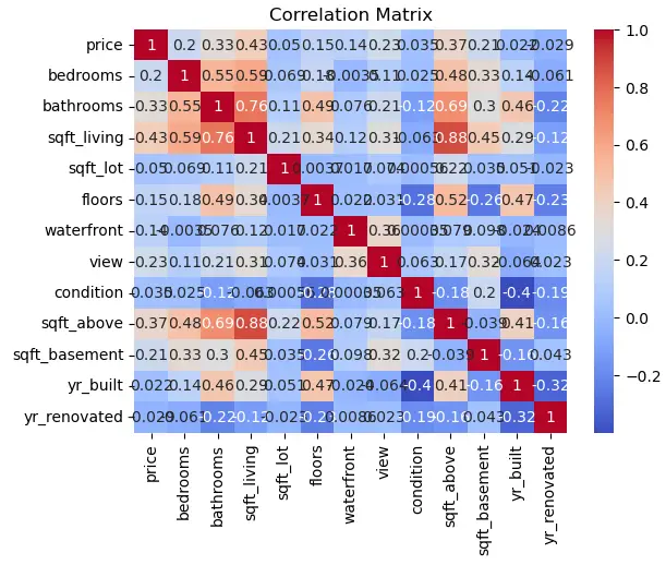
Step 2: Building the Linear Regression Model:
# Building the Linear Regression Model
model = LinearRegression()

# Fitting the model on the training data
model.fit(X_train, y_train)
Step 3: Model Evaluation:
# Model Evaluation
y_pred = model.predict(X_test)

# Mean Squared Error and R-squared for model evaluation
mse = mean_squared_error(y_test, y_pred)
r2 = r2_score(y_test, y_pred)

print("Mean Squared Error:", mse)
print("R-squared:", r2)
Mean Squared Error: 986869414953.98
R-squared: 0.03233518995632512
Step 4. Predictions and Visualization:
# Predictions and Visualization
# To visualize the predictions against actual prices, we'll use a scatter plot
plt.scatter(y_test, y_pred)
plt.xlabel("Actual Prices")
plt.ylabel("Predicted Prices")
plt.title("Actual Prices vs. Predicted Prices")
plt.show()

# We can also create a residual plot to check the model's performance
residuals = y_test - y_pred
plt.scatter(y_test, residuals)
plt.axhline(y=0, color='red', linestyle='--')
plt.xlabel("Actual Prices")
plt.ylabel("Residuals")
plt.title("Residual Plot")
plt.show()

# Lastly, let's use the trained model to make predictions on new data and visualize the results
new_data = [[3, 2, 1500, 4000, 1, 0, 0, 3]]
predicted_price = model.predict(new_data)

print("Predicted Price:", predicted_price[0])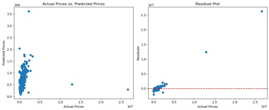
Predicted Price: 331038.9687692916
Conclusion
Linear regression is a powerful machine learning algorithm that can be applied to predict house prices accurately. By gathering and preprocessing relevant data, building and fine-tuning the model, and evaluating its performance, we can develop a valuable tool for the real estate industry. As technology advances further, machine learning models like linear regression continue to transform the way we make decisions, turning data into meaningful insights for a better future.
Find this tutorial on Github.